Usage¶

To use dvha-stats in a project:

Statistical data can be easily accessed with dvhastats.ui.DVHAStats class.

Getting Started¶

Before attempting the examples below, run these lines first:

>>> from dvhastats.ui import DVHAStats
>>> s = DVHAStats("your_data.csv")  # use s = DVHAStats() for test data

This assumes that your csv is formatted such that it contains one row per observation (i.e., wide format). If your csv contains multivariate data with one row per dependent value (i.e., narrow format), you can use dvhastats.utilities.widen_data(). See Reformatting CSV for an example.

Basic Plotting¶

>>> s.var_names
['V1', 'V2', 'V3', 'V4', 'V5', 'V6']

>>> s.get_data_by_var_name('V1')
array([56.5, 48.1, 48.3, 65.1, 47.1, 49.9, 49.5, 48.9, 35.5, 44.5, 40.3,
       43.5, 43.7, 47.5, 39.9, 42.9, 37.9, 48.7, 41.3, 47.1, 35.9, 46.5,
       45.1, 24.3, 43.5, 45.1, 46.3, 41.1, 35.5, 41.1, 37.3, 42.1, 47.1,
       46.5, 43.3, 45.9, 39.5, 50.9, 44.1, 40.1, 45.7, 20.3, 46.1, 43.7,
       43.9, 36.5, 45.9, 48.9, 44.7, 38.1,  6.1,  5.5, 45.1, 46.5, 48.9,
       48.1, 45.7, 57.1, 35.1, 46.5, 29.5, 41.5, 53.3, 45.3, 41.9, 45.9,
       43.1, 43.9, 46.1])

>>> s.show('V1')  # or s.show(0), can provide index or var_name

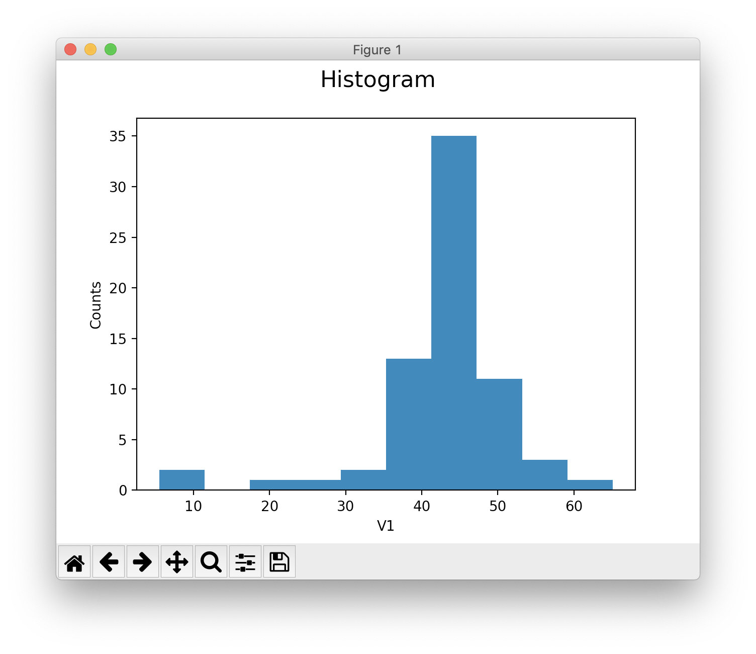
Histogram¶

Calculation with numpy.

>>> h = s.histogram('V1')
>>> hist, center = h.hist_data
>>> hist
array([ 2,  0,  0,  0,  0,  1,  1,  0,  1,  0,  5,  4,  9, 15, 17, 10,  1,
    1,  1,  0,  1]
>>> center
array([ 6.91904762,  9.75714286, 12.5952381 , 15.43333333, 18.27142857,
       21.10952381, 23.94761905, 26.78571429, 29.62380952, 32.46190476,
       35.3       , 38.13809524, 40.97619048, 43.81428571, 46.65238095,
       49.49047619, 52.32857143, 55.16666667, 58.0047619 , 60.84285714,
       63.68095238])

Calculation with matplotlib.

>>> s.show(0, plot_type="hist")  # histogram recalculated using matplotlib

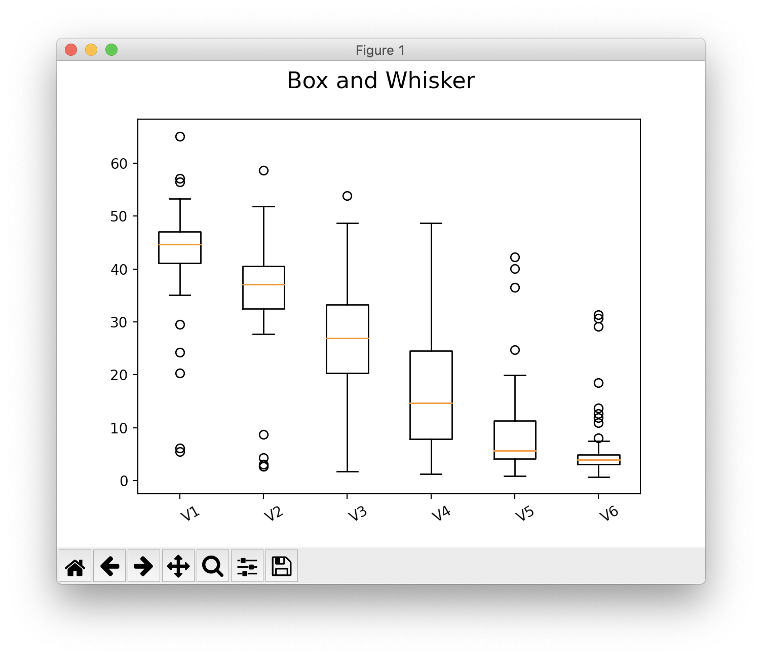
Box & Whisker Plot¶

Calculation with matplotlib

>>> s.show(0, plot_type="box")

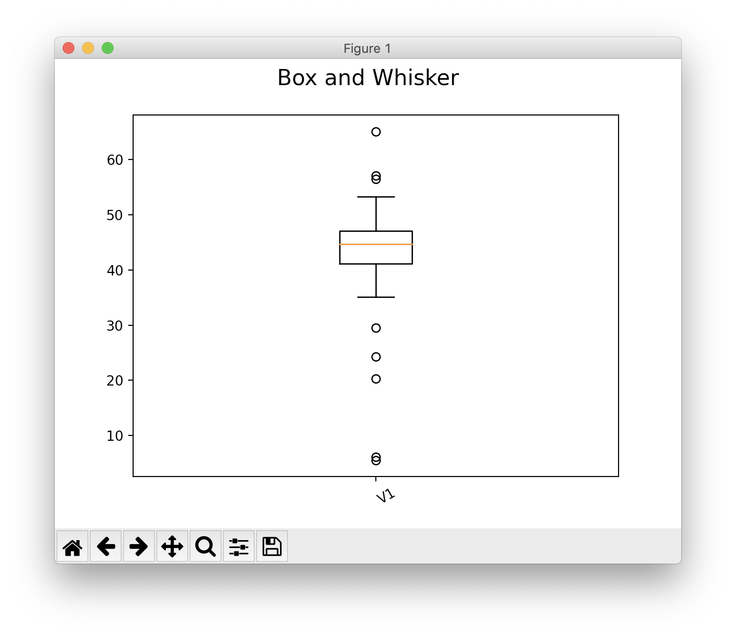
>>> s.show(plot_type="box")

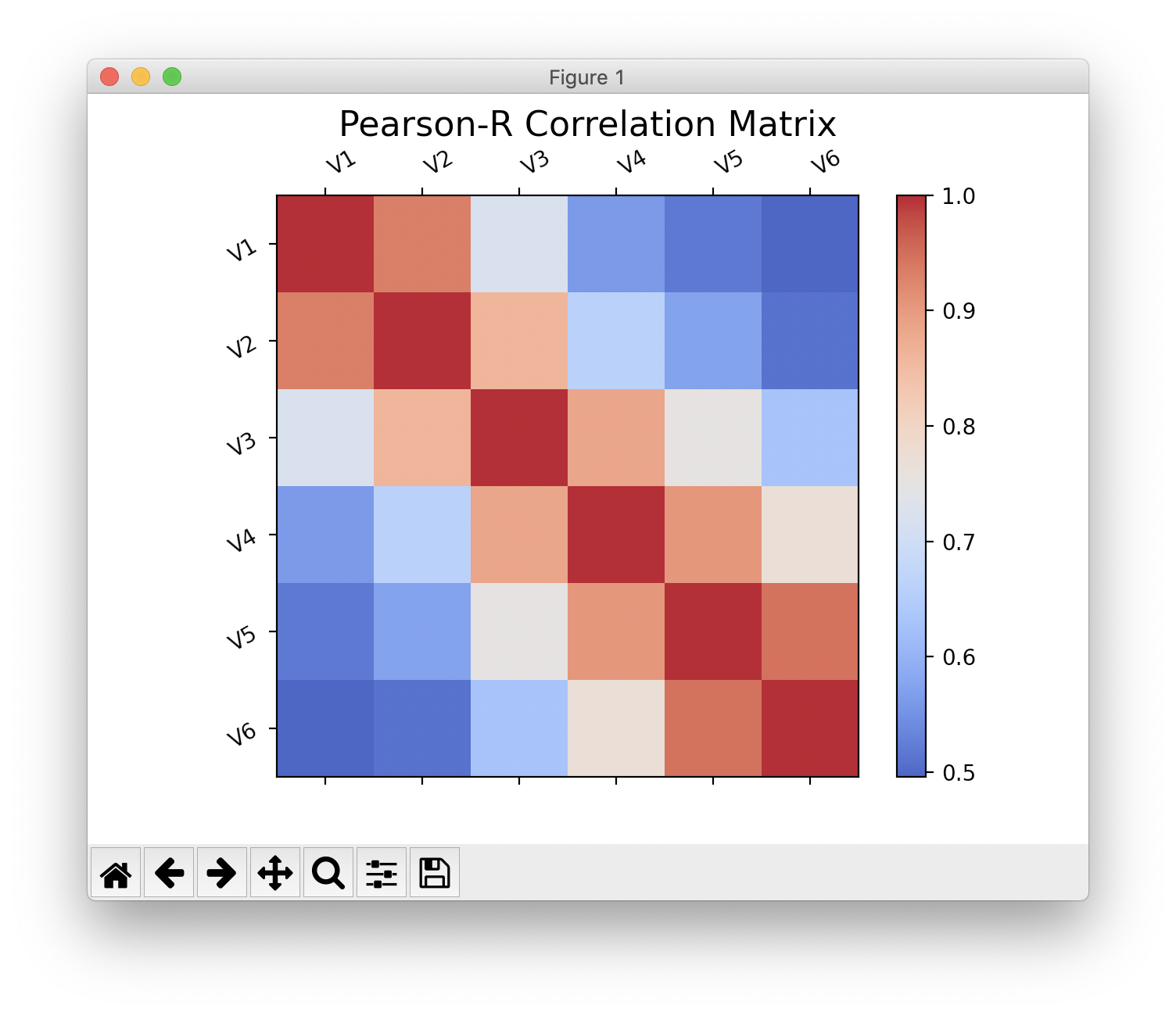
Pearson-R Correlation Matrix¶

Calculation with scipy.

>>> pearson_mat = s.correlation_matrix()
>>> pearson_mat.corr  # correlation array
array([[1.        , 0.93160407, 0.72199862, 0.56239953, 0.51856243, 0.49619153],
       [0.93160407, 1.        , 0.86121347, 0.66329274, 0.5737434 , 0.51111648],
       [0.72199862, 0.86121347, 1.        , 0.88436716, 0.7521324 ,  0.63030588],
       [0.56239953, 0.66329274, 0.88436716, 1.        , 0.90411476, 0.76986654],
       [0.51856243, 0.5737434 , 0.7521324 , 0.90411476, 1.        , 0.9464186 ],
       [0.49619153, 0.51111648, 0.63030588, 0.76986654, 0.9464186 , 1.        ]])
>>> pearson_mat.p  # p-values
array([[0.00000000e+00, 3.70567507e-31, 2.54573222e-12, 4.92807604e-07, 5.01004755e-06, 1.45230750e-05],
       [3.70567507e-31, 0.00000000e+00, 2.27411745e-21, 5.28815300e-10, 2.55750429e-07, 7.19979746e-06],
       [2.54573222e-12, 2.27411745e-21, 0.00000000e+00, 7.41613930e-24, 9.37849945e-14, 6.49207976e-09],
       [4.92807604e-07, 5.28815300e-10, 7.41613930e-24, 0.00000000e+00, 1.94118606e-26, 1.06898267e-14],
       [5.01004755e-06, 2.55750429e-07, 9.37849945e-14, 1.94118606e-26, 0.00000000e+00, 1.32389842e-34],
       [1.45230750e-05, 7.19979746e-06, 6.49207976e-09, 1.06898267e-14, 1.32389842e-34, 0.00000000e+00]])
>>> pearson_mat.show()

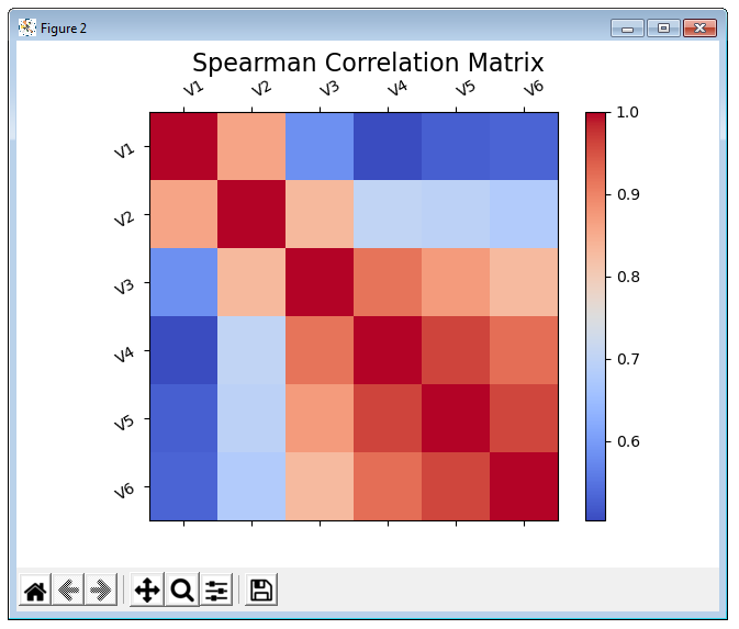
Spearman Correlation Matrix¶

Calculation with scipy.

>>> spearman_mat = s.correlation_matrix("Spearman")
>>> spearman_mat.show()

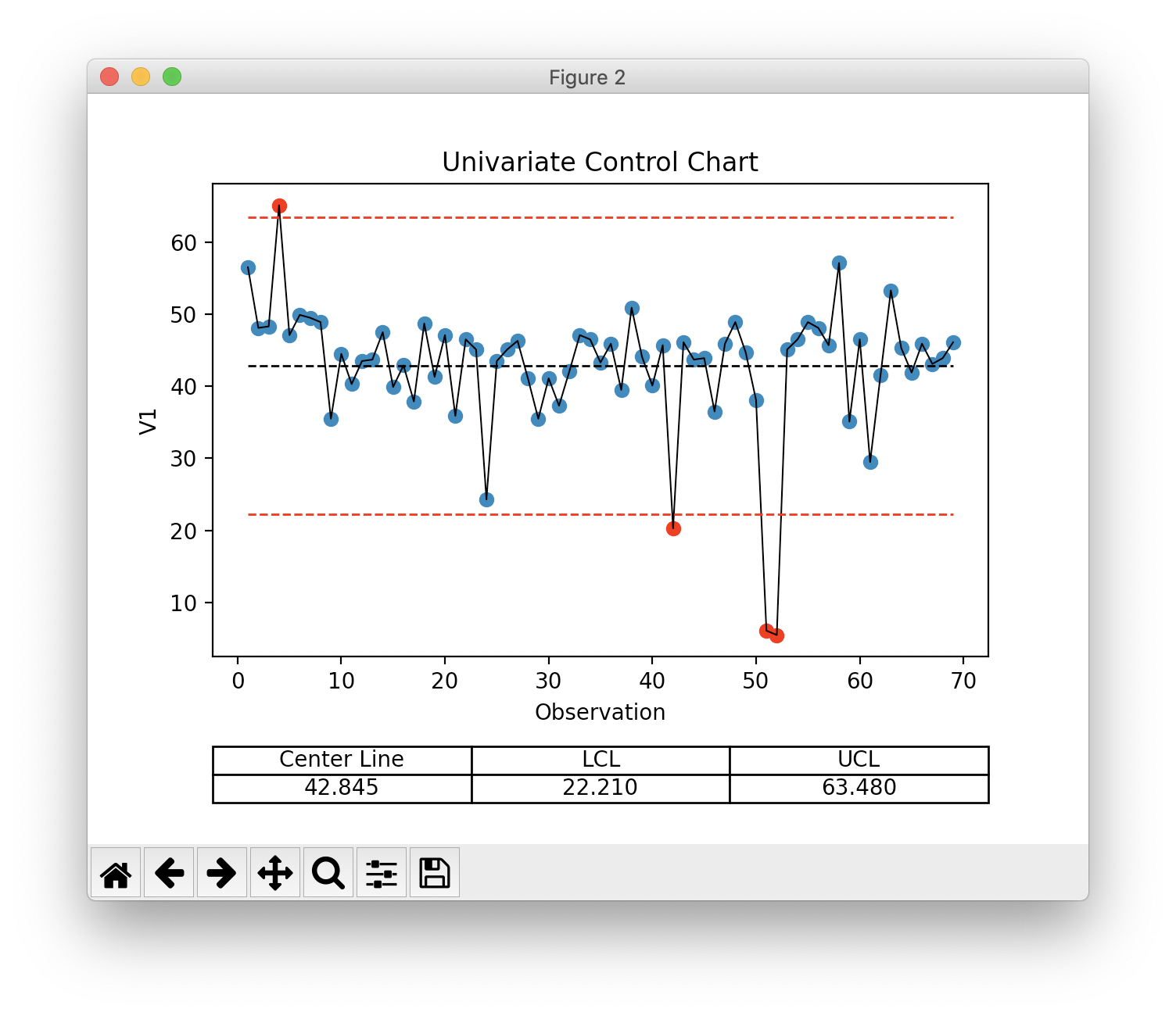
Univariate Control Chart¶

>>> ucc = s.univariate_control_charts()
>>> ucc['V1']
center_line: 42.845
control_limits: 22.210, 63.480
out_of_control: [ 3 41 50 51]

>>> ucc['V1'].show()  # or ucc[0].show(), can provide index or var_name

Multivariate Control Chart¶

>>> ht2 = s.hotelling_t2()
>>> ht2
Q: [ 5.75062092  3.80141786  3.67243782 18.80124504  2.03849294 18.15447155
     4.54475048 10.40783971  3.60614333  4.03138994  6.45171623  4.60475303
     2.29185301 15.7891342   3.0102578   6.36058098  5.56477106  3.92950273
     1.70534379  2.14021007  7.3839626   1.16554558  7.89636669 20.13613585
     3.76034723  0.93179106  2.05542886  2.65257506  1.31049764  1.59880892
     2.13839258  3.33331329  4.01060102  2.71837612 10.0744586   4.50776545
     1.87955428  7.13423455  4.1773818   3.70446025  3.49570988 11.52822658
     5.874624    2.34515306  2.71884639  2.58457841  3.2591779   4.69554484
     9.1358149   2.64106059 21.21960037 22.6229493   1.55545875  2.29606726
     3.96926714  2.69041382  1.47639788 17.83532339  4.03627833  1.78953536
    15.7485067   1.56110637  2.53753085  2.04243193  6.20630748 14.39527077
     9.88243129  3.70056854  4.92888799]
center_line: 5.375
control_limits: 0, 13.555
out_of_control: [ 3  5 13 23 50 51 57 60 65]

>>> ht2.show()ht

Box-Cox Transformation (for non-normal data)¶

Calculation with scipy.

>>> bc = s.box_cox_by_index(0)
>>> bc
array([3185.2502073 , 2237.32503551, 2257.79294148, 4346.90639712,
       2136.50469314, 2425.19594298, 2382.73410297, 2319.80580872,
       1148.63472597, 1886.15962058, 1517.3226398 , 1794.37742725,
       1812.53465647, 2176.52932216, 1484.4619302 , 1740.50195077,
       1326.0093692 , 2299.03324672, 1601.1904051 , 2136.50469314,
       1177.23656545, 2077.22485894, 1942.42664844,  499.72380601,
       1794.37742725, 1942.42664844, 2057.66647538, 1584.22036354,
       1148.63472597, 1584.22036354, 1280.36568471, 1670.05579771,
       2136.50469314, 2077.22485894, 1776.31962594, 2018.85154453,
       1451.99231252, 2533.13894266, 1849.14775291, 1500.84335095,
       1999.59482773,  336.62160027, 2038.20873211, 1812.53465647,
       1830.79140224, 1220.85798302, 2018.85154453, 2319.80580872,
       1904.81531264, 1341.41740006,   23.64034973,   18.74313335,
       1942.42664844, 2077.22485894, 2319.80580872, 2237.32503551,
       1999.59482773, 3259.95515527, 1120.41519999, 2077.22485894,
        764.99904232, 1618.25887705, 2802.6765172 , 1961.38246534,
       1652.69148146, 2018.85154453, 1758.36116355, 1830.79140224,
       2038.20873211])

Multivariate Control Chart (w/ non-normal data)¶

>>> ht2_bc = s.hotelling_t2(box_cox=True)
>>> ht2_bc.show()

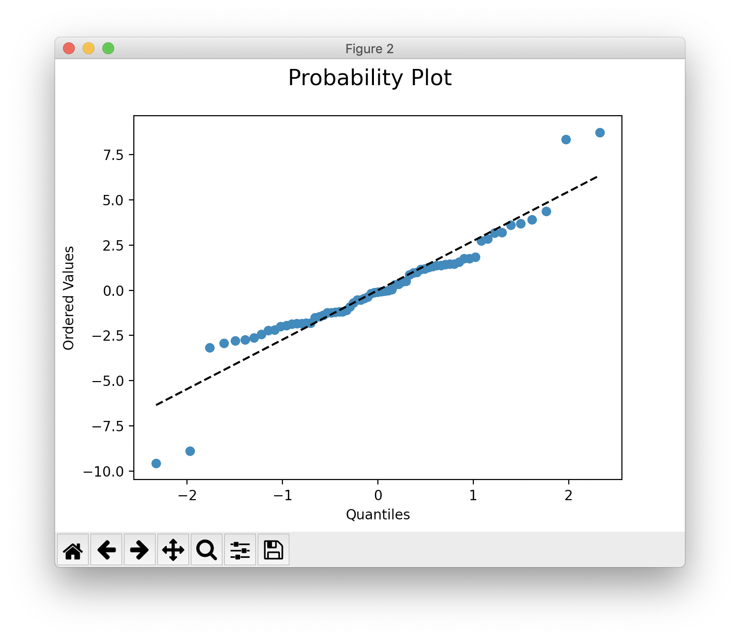
Multi-Variable Linear Regression¶

Calculation with sklearn.

>>> mvr = s.linear_reg("V1")
>>> mvr

Multi-Variable Regression results/model
R²: 0.906
MSE: 7.860
f-stat: 121.632
f-stat p-value: 1.000
+-------+------------+-----------+---------+---------+
|       |       Coef | Std. Err. | t-value | p-value |
+-------+------------+-----------+---------+---------+
| y-int |  1.262E+01 | 1.326E+00 |   9.518 |   0.000 |
|   V2  |  1.107E+00 | 7.547E-02 |  14.664 |   0.000 |
|   V3  | -4.442E-01 | 1.135E-01 |  -3.914 |   0.000 |
|   V4  |  1.786E-01 | 1.340E-01 |   1.333 |   0.187 |
|   V5  | -1.789E-01 | 2.538E-01 |  -0.705 |   0.483 |
|   V6  |  2.833E-01 | 2.355E-01 |   1.203 |   0.233 |
+-------+------------+-----------+---------+---------+

>>> mvr.show()

>>> mvr.show("prob")

>>> mvr2 = s.linear_reg("V1", back_elim=True)
>>> mvr2

Multi-Variable Regression results/model
R²: 0.903
MSE: 8.096
f-stat: 202.431
f-stat p-value: 1.000
+-------+------------+-----------+---------+---------+
|       |       Coef | Std. Err. | t-value | p-value |
+-------+------------+-----------+---------+---------+
| y-int |  1.276E+01 | 1.321E+00 |   9.656 |   0.000 |
|   V2  |  1.070E+00 | 6.700E-02 |  15.967 |   0.000 |
|   V3  | -3.318E-01 | 6.852E-02 |  -4.843 |   0.000 |
|   V6  |  2.000E-01 | 7.542E-02 |   2.652 |   0.010 |
+-------+------------+-----------+---------+---------+

Risk-Adjusted Control Chart¶

>>> ra_cc = s.risk_adjusted_control_chart("V1", back_elim=True)
>>> ra_cc.show()

Principal Component Analysis (PCA)¶

Calculation with sklearn.

>>> pca = s.pca()
>>> pca.feature_map_data
array([[ 0.35795147,  0.44569046,  0.51745294,  0.48745318,  0.34479542, 0.22131141],
       [-0.52601728, -0.51017406, -0.02139406,  0.4386136 ,  0.43258992, 0.28819198],
       [ 0.42660699,  0.01072412, -0.5661977 , -0.24404558,  0.39945093, 0.52743943]])
>>> pca.show()

Reformatting CSV¶

Below is an example of how to reformat a “narrow” csv (one row per dependent variable value) to a “wide” format (one row per observation). Please see dvhastats.utilities.widen_data for additional documentation.

Let’s assume the contents of your csv file looks like:

patient,plan,field id,image type, date, DD(%), DTA(mm),Threshold(%),Gamma Pass Rate(%)
ANON1234,Plan_name,3,field,6/13/2019 7:27,3,2,10,99.94708217
ANON1234,Plan_name,3,field,6/13/2019 7:27,3,3,5,99.97934552
ANON1234,Plan_name,3,field,6/13/2019 7:27,3,3,10,99.97706894
ANON1234,Plan_name,3,field,6/13/2019 7:27,2,3,5,99.88772435
ANON1234,Plan_name,4,field,6/13/2019 7:27,3,2,10,99.99941874
ANON1234,Plan_name,4,field,6/13/2019 7:27,3,3,5,100
ANON1234,Plan_name,4,field,6/13/2019 7:27,3,3,10,100
ANON1234,Plan_name,4,field,6/13/2019 7:27,2,3,5,99.99533258

We can see that all data here is of the same patient, plan, and date. In this example, we want to evaluate the variation of Gamma Pass Rate(%) as a function of DD(%), DTA(mm), and Threshold(%). So, in this context, we really only want two rows of data, one for each field id (i.e., 3 or 4).

>>> from dvhastats.utilities import csv_to_dict, widen_data
>>> data_dict = csv_to_dict("path_to_csv_file.csv")
>>> uid_columns = ['patient', 'plan', 'field id']  # only field id really needed in this case
>>> x_data_cols = ['DD(%)', 'DTA(mm)', 'Threshold(%)']
>>> y_data_col = 'Gamma Pass Rate(%)'
>>> wide_data = widen_data(data_dict, uid_columns, x_data_cols, y_data_col)
>>> wide_data
    {'uid': ['ANON1234Plan_name3', 'ANON1234Plan_name4'],
     '2/3/5': ['99.88772435', '99.99533258'],
     '3/2/10': ['99.94708217', '99.99941874'],
     '3/3/10': ['99.97706894', '100'],
     '3/3/5': ['99.97934552', '100']}